I recently started to do some work with NSS (National Student Survey) data, which are available from the HEFCE website in the form of Excel workbooks. To get the data I wanted, I started copying and pasting, but I quickly realised how hard it was going to be to be sure that I hadn’t made any mistakes. (Full disclosure: it turns out that actually I did make some mistakes, e.g. once I left out an entire row because I hadn’t noticed that it wasn’t selected.) Using a programming language such as R to create a script to import data requires much more of an investment of time upfront than diving straight in and beginning to copy and paste but the payoff is that once your script works, you can use it over and over again – which is why I now have several years’ worth of NSS data covering all courses and institutions, from which I can quite easily pull out whichever numbers I want using a dplyr filter statement (as long as I am prepared to take account of irregularities e.g. in institutions’ names from one year to the next – which would also be necessary when doing things by point-and-click).
For example, looking at how all institutions performed in my particular discipline with regard to the four NSS questions relating to teaching quality, I can see that Media Studies at the University of the West of England managed the quite remarkable feat of rising from 68th place in 2015 to 2nd place in 2016 before falling back to 53rd place in 2017. To visualise only these four questions in relation to this subject at this institution over the whole time period for which I have data, I can filter out everything relating to other disciplines and other institutions with a single statement, and then use ggplot to represent each of the four variables that I’m interested in with a different coloured line:
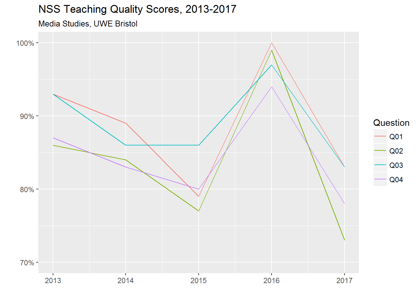
How could such a dramatic rise and fall occur? Maybe someone who still works at UWE would be better placed to explain. But the general question of what drives student perceptions of teaching quality is one that I’m interested to explore as a researcher – and I’ll be posting thoughts and findings here as and when.
In the meantime, here’s my code, presented as an example of how the automation of error-prone tasks can take some of the uncertainty out of the research process. You probably aren’t interested in working with this particular dataset, but you may have other datasets that you would like to deal with in the same way. Yes, it looks complicated if you’re not used to scripting – but the code is actually quite simple, and the thing is that I was able to build it up iteratively, by adding statements, running the script as a whole, noticing what went wrong, and then fixing whatever it was, one step at a time. (The code is very heavily commented, to give a non-coder an idea of what those steps were and what sort of thinking is typically involved in taking a code-based rather than point-and-click-based approach to data importing etc.)
Of course, there were bugs that had to be fixed. But now that the code works, it works. This is the difference between doing things by hand – where I may make new errors when I go back to fix the old ones – and automating the tasks involved – where errors in the automation can be progressively ironed out until none remain. So while I originally wrote that script to work with the JACS subject level 3 spreadsheets for 2013-2017, I can easily (a) add more years just by downloading the relevant Excel files, putting them in the same folder, and adding the filenames to the filename.years variable, or (b) use a different JACS subject level just by changing the JACS.level variable from 3 to 1 or 2. Either of these done, I can then run the same script to create the same analyses and visualisations of a different or larger dataset. Neat, huh?
This example’s in R, but you don’t have to learn R to do this sort of thing. For example, you can also script in SPSS using the Syntax Editor (I’ve never used SPSS at all, but my experience is that – with a few notable exceptions – any software tool that large numbers of people and institutions pay for will typically raise your blood pressure by less than the nearest Open Source equivalent). Regardless of which tool you use, the more you script and the less you click, the better documented and the more reproducible your work will be – which means that (apart from anything else) you’ll be more likely to be able to make changes to your dataset or to the procedures used at any stage of your analysis and yet still re-run everything without the effort and uncertainty of trying to remember which exact steps you went through last time because all the steps will be right there. If you get things done by adding commands to a script rather than by clicking on buttons and menu options, and if you are disciplined about saving your script regularly and making clear which is the most up-to-date version of it (which you can achieve through version control, e.g. with git, but which you can also achieve simply by naming your files helpfully and keeping them organised in folders), and especially if you comment your code to make it easier for another person (including your future self) to understand, then your work will be its own documentation and you will be able to refine or repeat it at any point – including at that awful point when a peer reviewer demands that you start your analysis again with some particular modification to your dataset or procedure. And while this particular script does nothing but import data, you can also write code to run regressions, create tables, plot visualisations, etc, which means that a whole project can be contained in a single file that’s small enough to send by email.
# Code to import spreadsheets exported from the
# Excel workbooks available from the HEFCE website,
# saved in a sub-directory called `excel-files`

# N.B. In R, anything beginning with a `#` sign is a
# comment for the human reader of the code.

# Put the filenames of the spreadsheets and the years
# those spreadsheets represent into a variable. If
# we want to add more years later, we just have to
# save the files in the same directory and add their
# names here
filename.years <- c('NSS_taught_all13.xlsx' = 2013,
                    'NSS_taught_all14-new.xlsx' = 2014,
                    'NSS_taught_all15.xlsx' = 2015,
                    'NSS_taught_all16.xlsx' = 2016,
                    'NSS_taught_all17.xlsx' = 2017)

# Variable recording which JACS level we're interested
# in so that only the correct spreadsheets are
# loaded from the workbooks
JACS.level <- 3

# Put the names of all the columns we're interested in
# into another variable called 'cols.to.keep'
cols.to.keep <- c('Year', 'Institution', 'Subject', 'Level',
                  'Question Number', 'Actual value', 'Response',
                  'Sample Size', 'Two years aggregate data?')

# Define a function to load one spreadsheet and get it
# into a standard form so it can be merged with
# others. To use this function, we'll call it with a
# specific year and it will load the spreadsheet for
# that year. The function will be called
# load.nss.file:
load.nss.file <- function(year) {
  # Combine the name of the directory name where
  # the sheets are saved with the filename
  # corresponding to the year the function has
  # been called with
  fp <- paste(c('excel-files', names(year)), collapse = '/')
  # Load the correct spreadsheet using read_excel from
  # readxl; leave out the first three rows; use
  # the values in the next row as column names;
  # store the data in the variable 'd'
  d <- read_excel(fp, sheet = JACS.level + 2,
                  skip = 3,
                  col_names = TRUE
                  )
  # Create a new column for the year. This will be
  # the same in every row of the current spreadsheet,
  # but will be useful once we start amalgamating
  # spreadsheets
  d$Year <- year
  # Are all the columns we want actually in this
  # spreadsheet? Find out whether each one is there
  # and store the resulting vector in the variable
  # 'usable.cols'
  usable.cols <- cols.to.keep %in% colnames(d)
  # Now find out the names of the columns we want
  # that are missing from this spreadsheet. Put their
  # names into the variable 'missing.cols'
  missing.cols <- cols.to.keep[!usable.cols]
  # Loop through all the missing column names. For
  # each one, create a new column and fill it with
  # NAs (the symbol used to show that a value is
  # missing)
  for (x in missing.cols) {
    d[x] <- NA
  }
  # Select the columns we want, and return a data
  # frame containing only those. Note that this also
  # re-orders the columns to match the vector of names
  # in the 'cols.to.keep' variable
  d[cols.to.keep]
}

# Now that we've got our function, it's time to use
# it to load all the spreadsheets we want into memory
# and keep them in a single data frame. Here goes!

# Create empty variable called `d`. The data is going
# in there. (In R, it's standard practice to call data
# frames `d` if you can't think of anything better. It
# doesn't matter that we have a variable called `d` in
# the function above; R won't get them mixed up.)
d <- NA

# Now loop through all the names in `filename.years`
# one by one, always referring to the name we're
# currently dealing with as `x`:
for (x in names(filename.years)) {
  # Call the above-defined load.nss.file function with
  # the year corresponding to one name (stored in the
  # variable `x`), and store the data frame
  # that it returns in the variable 'loaded.file':
  loaded.file <- load.nss.file(filename.years[x])
  # Check whether the `d` variable has a data frame
  # stored in it yet:
  if (!is.data.frame(d)) {
    # If not, this is the first time we've been
    # around the loop, so store the data frame from
    # 'loaded.file' in it
    d <- loaded.file
  } else {
    # Otherwise, add the rows from the 'loaded.file'
    # data frame to the bottom of the data frame
    # currently stored in `d`:
    d <- rbind(d, loaded.file)
  }
  # This is the end of the loop, so R will go back
  # to the beginning if there are any more names to
  # loop through.
}

# Now forget the 'loaded.file' variable, the last
# version of which will stay in memory otherwise:
rm(loaded.file)

# Change all values into the forms we want to work
# with (note that 'Two years aggregate data?' is either
# 'Y' or blank; we will want TRUE or FALSE). We can
# do this with the transmute function from the dplyr
# package, which also enables us to simultaneously
# rename and reorder the columns and to discard
# the ones we're not interested in
d <- transmute(
  d,
  Institution = factor(Institution),
  Subject = factor(Subject),
  Level = factor(Level),
  Year = as.numeric(Year),
  Question = `Question Number`,
  Agree = as.numeric(`Actual value`),
  Respondents = as.numeric(Response),
  Cohort = as.numeric(`Sample Size`),
  Aggregate = !is.na(`Two years aggregate data?`))

# Now that's done, we can think about transforming
# the data further. Later I will change from
# HEFCE's 'long' format (one question result per line)
# to a tidier 'wide' format (all question results for
# a single course in a single year on one line)
# using dcast from the reshape2 package. However,
# missing data in the Question column would cause that
# function call to fail, so now we get rid of any
# such rows with filter (another dplyr function):
d <- filter(
  # Work with the existing `d` data frame
  d,
  # Only keep rows if they do NOT have an NA
  # in the Question column
  !is.na(Question)
)

# And there we are.